Neural networks

Alexandre Boulch

IOGS - ATSI


Outline

  • Introduction
  • The artificial neuron
    • Formulation
    • Stochastic gradient descent
  • The multi-layer perceptron
    • Stacking neurons
    • Chain rule
     

Motivation

Simple problem:

Predict if Bob will like a movie given Alice's grade

Hypothesis:

Linear problem


Motivation

Simple problem:
Predict if Bob will like a movie given Alice's grade

Hypothesis:
A simple threshold:


center


Motivation

Simple problem:
Predict if Bob will like a movie given Alice's grade

Hypothesis:
A simple threshold


center


Motivation

Simple problem:
Predict if Bob will like a movie given Alice's and Carol's grades

Hypothesis:
An affine function


center


Motivation

More complicated problem:
Predict if Bob will like a movie given a large user database

Hypothesis:
An affine function


Motivation

More complicated problem:
Predict if Bob will like a movie given a large user database

Hypothesis:
Non-affine function ?

inputs, parameters, function


Motivation

Ideally

  • General machine learning architectures / bricks
    • use the same approach for various problems
  • Learn the parameters
    • Use data to automatically extractknowledge

Neural networks

  • Currently one of the most efficient approach for machine learning
     

Artificial neuron


Historical Background

  • 1958: Rosenbalt, perceptron
  • 1965: Ivakhenko and Lapa, neural networks with several layers
  • 1975-1990: Backpropagation, Convolutional Neural Networks
  • 2007+: Deep Learning era (see Deep Learning sesion)
    • Large convolutional neural networks
    • Transformers
    • Generative models
    • "Foundation models"
    • ...
     

Bio inspired model

  • The brain is made of neurons.
  • Receive, process and transmit action potential.
  • Multiple recievers (dentrites), single transmitter (axon)
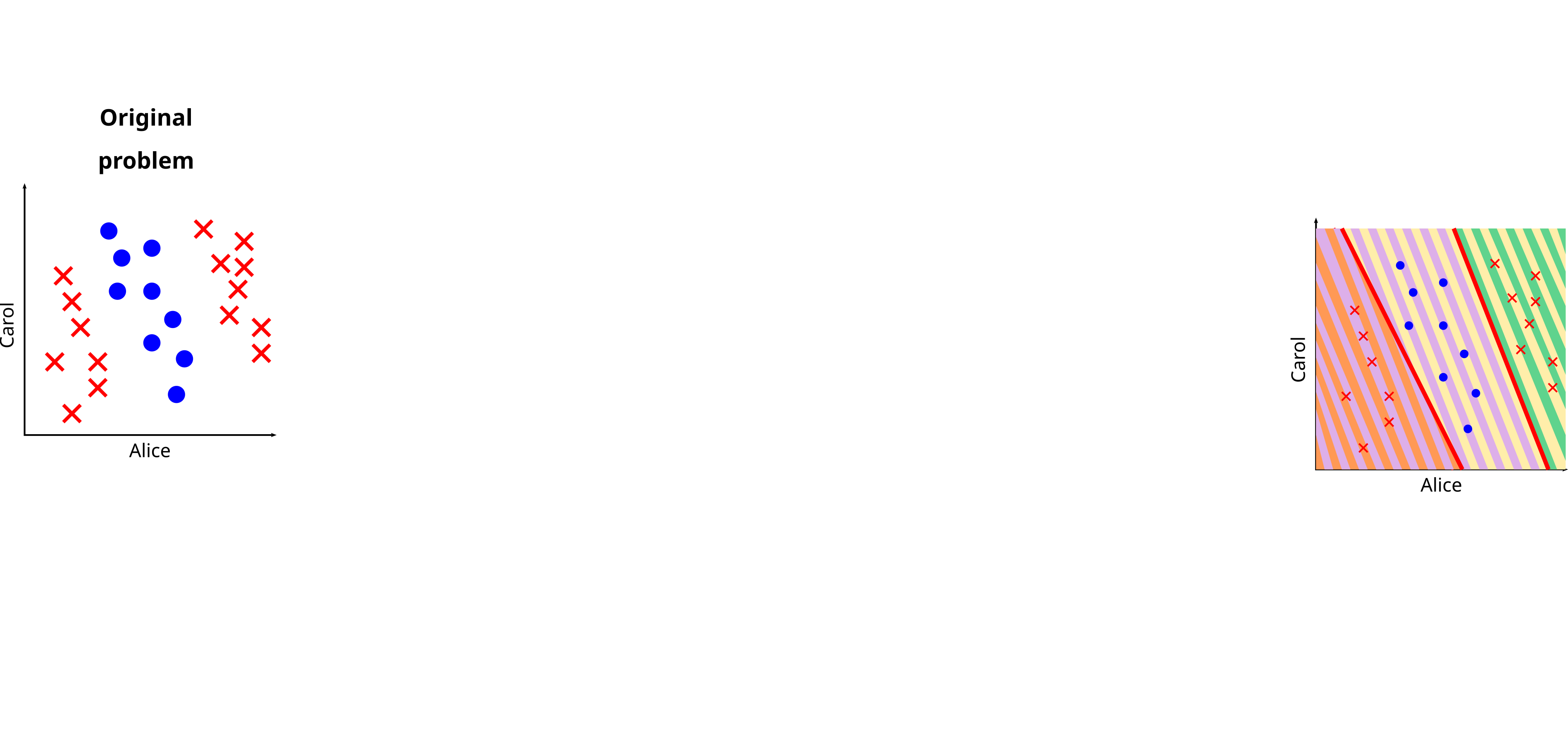
image wikipedia
     

Formulation

A simple model of the neuron: activation level is the weighted sum of the inputs


  • the input vector
  • the weight matrix
  • the bias
  • the output
  • the activation function
1958 : Rosenbalt, perceptron
     

Back to example

Simple problem:
Predict if Bob will like a movie given Alice's and Carol's grades

Hypothesis:
An affine function

It can be modeled with a single neuron with:


Geometric interpretation of the neuron


is an hyperplan of , with the dimension of the space.

The sign of activation defines on which side of lies .

The artificial neuron linear decision.

Previous course on SVM: the SVM was originally formulated using neurons.


Limitations

center


Limitations

center


Limitations

center


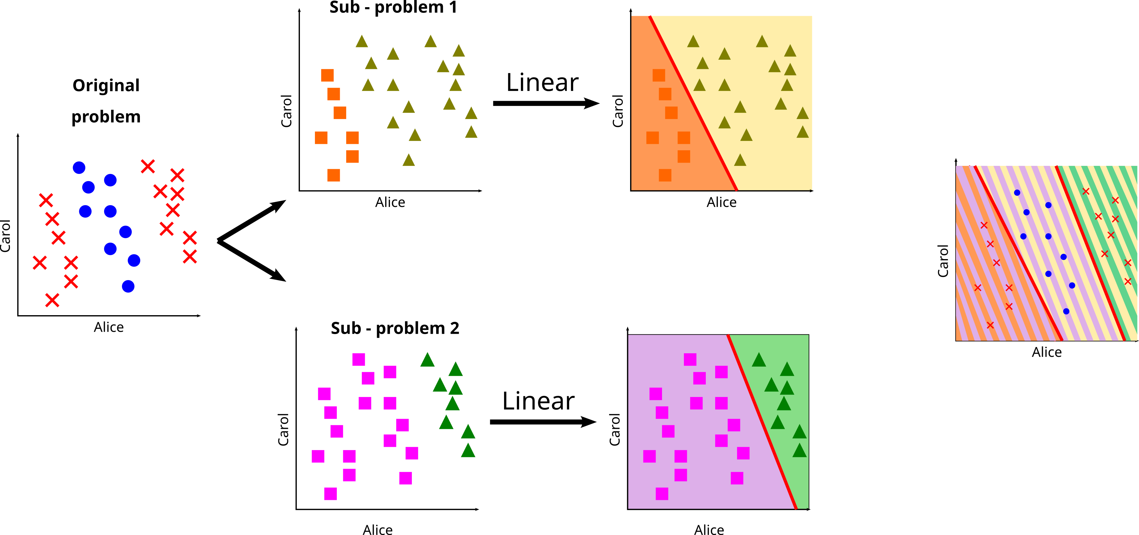
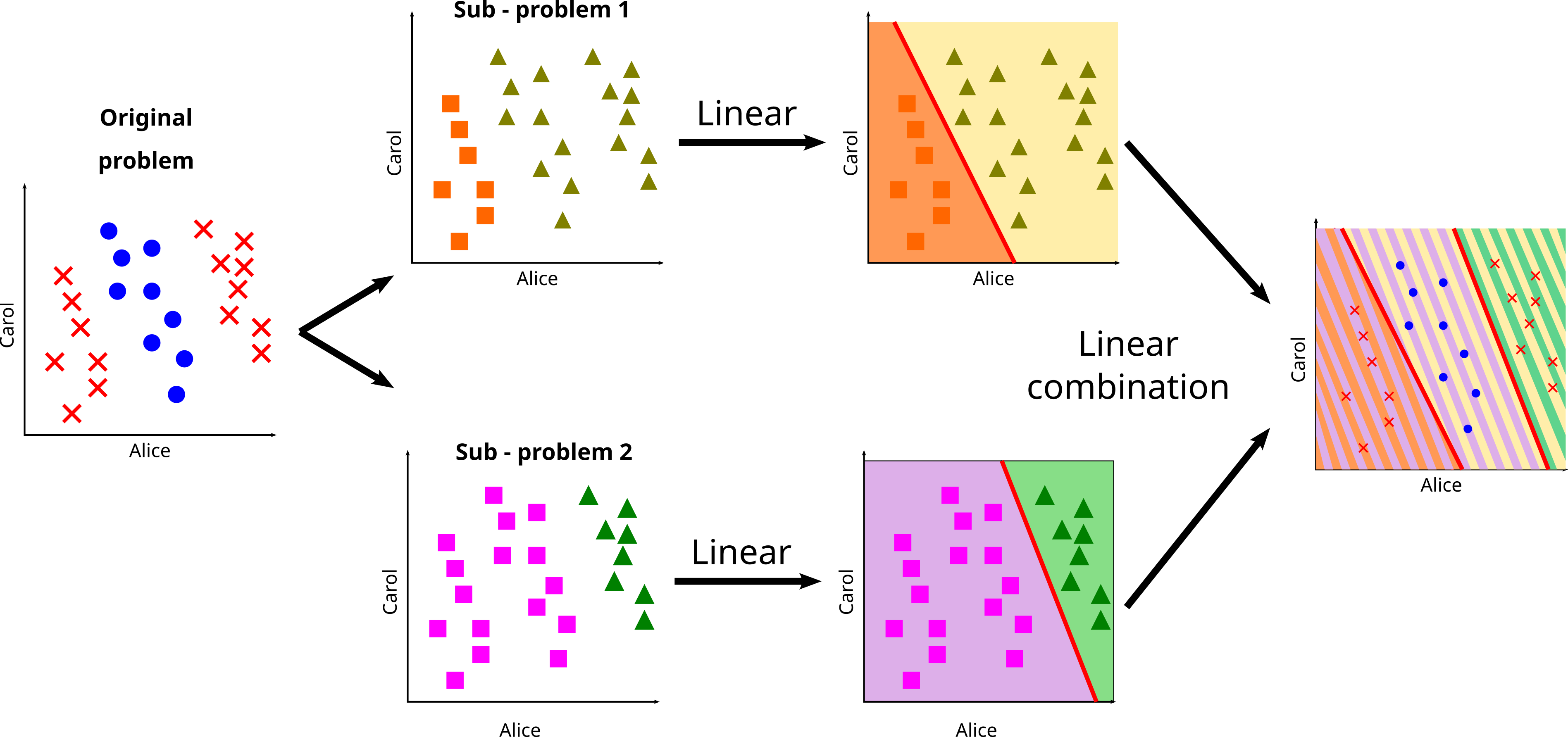
Possible solution: using multiple stacked neurons

center


Universal approximation theorem

Arbitrary width

Multilayer feed-forward networks with as few as one hidden layer are universal approximators

  • Cybenko (1989) for sigmoid activation functions
  • Hornik et al. (1989) for 1 hidden layer
  • Hornik (1991) any choice of the activation function

Arbitrary depth

  • Gripenberg (2003)
  • Yarotsky (2017), Lu et al (2017)
  • Hanin (2018)
  • Kidger (2020)
     

Neural networks in practice

Network design

  • high neuron number: very computationally expensive
  • prefer stacking more layers

Optimization

  • several parameters (probably many)
  • automatic optimization
  • gradient descent
     

Stochactic gradient descent


Optimizing the parameters

Objective

Find and such that:

for , the set of movies.


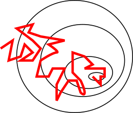
Gradient descent


Objective

Reach the bottom of the valley


Gradient descent


Objective

Reach the bottom of the valley


Gradient descent

Minimizing an objective function


Gradient descent

For every smooth function

i.e., following the opopsite direction of the gradient leands to a local minimum of the function.


Gradient descent

An iteratieve agorithm:

is the learning rate.

must be continuous and differentiable almost everywhere.


Gradient descent

center

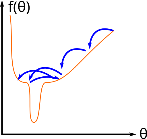
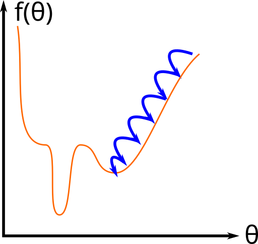
Too high learning rate.

center

Too low learning rate.


Back to example

Simple problem:
Predict if Bob will like a movie given Alice's and Carol's grades

Hypothesis:
An affine function

Problem

Sign function is:-

  • Zero-gradient everywhere
  • Not differentiable at 0
     

Objective / loss function

We need a function to compare predictions and ground truth.

A function such that:

  • it takes 0 values if
  • it is differentiable
  • it increases along with the "difference" between the and

Possibilities:

  • Squared differences:
  • Cross entropy (for categorical loss)
  • ...
     

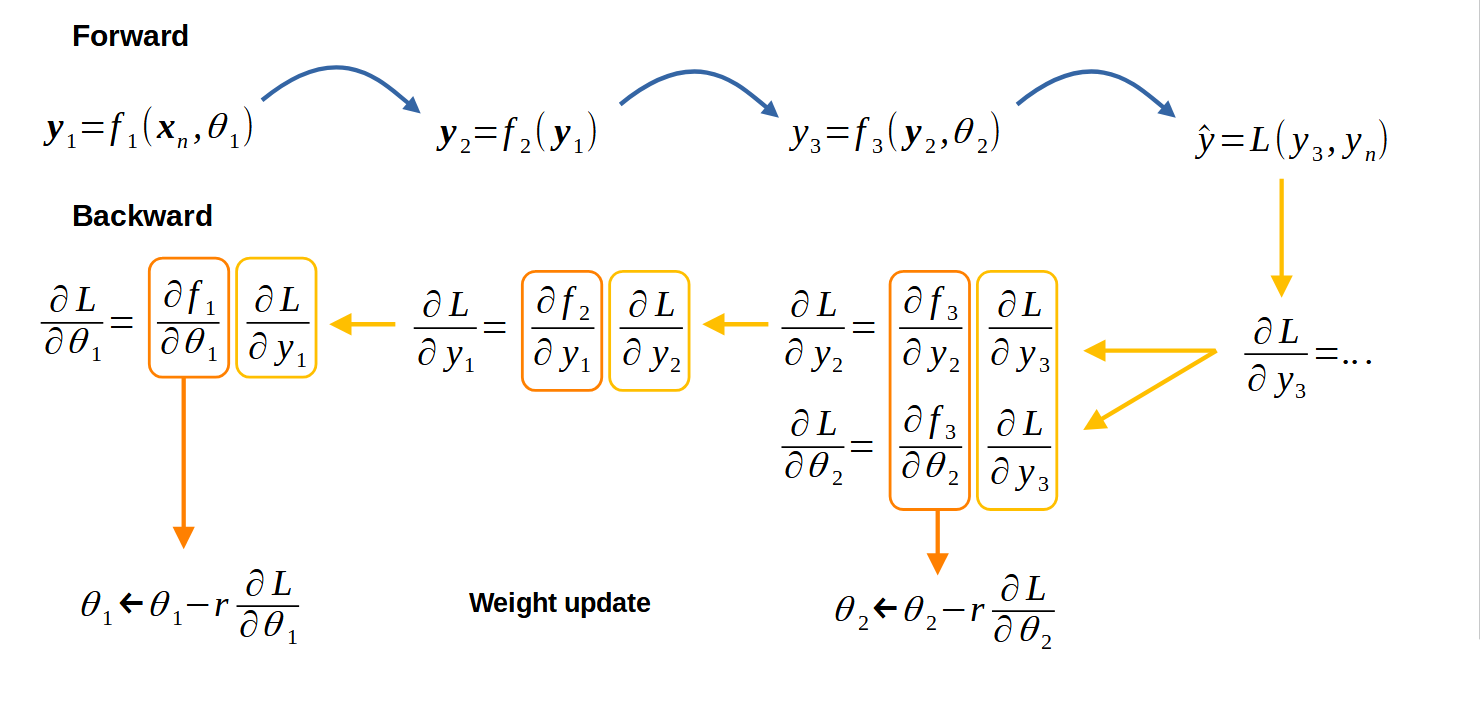
Optimization

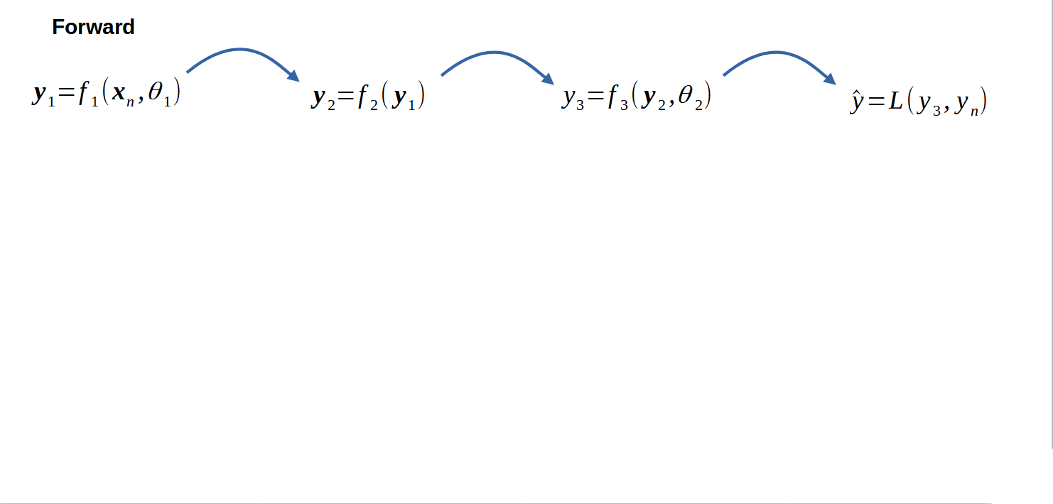
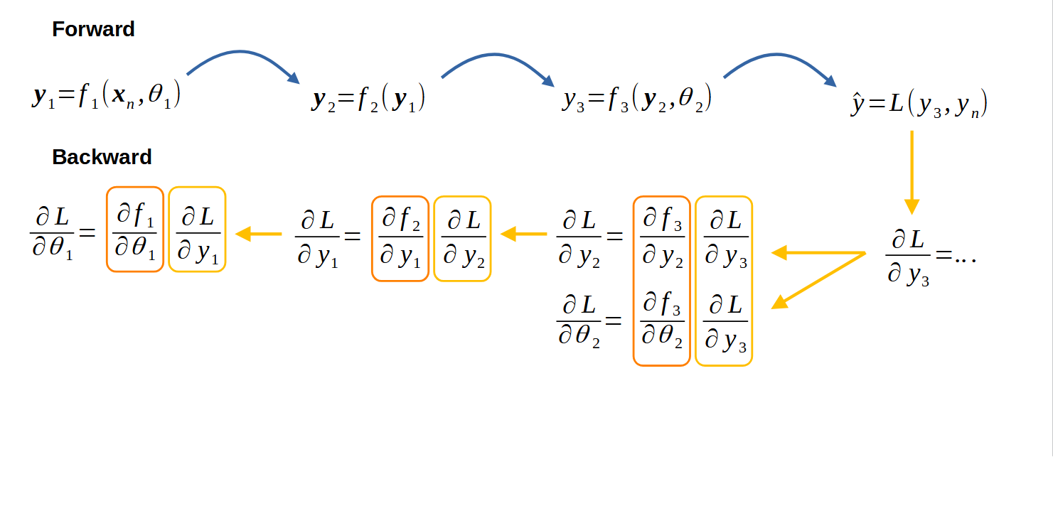
Forward

Iteratively compute the output of the network

Backward

Itertatively compute the derivatives starting from the output

Weight update

Update weights according to learning rate.


Mean Squared Differences

Loss function

Single neuron model

Derivatives:


Mean Squared Differences

Loss function

Single neuron model

Derivatives is computed at prediction time:


Mean Squared Differences

Loss function

Two neurons model

Derivatives:

We do not want to explicitely compute the loss function.


Chain rule

In practice, we make an intensive use of the chain rule:

or for three functions:


Chain rule applied to neural networks

center


Chain rule applied to neural networks

center


Chain rule applied to neural networks

center


Code architecture

class Module: 
  def __init__(self, …): 
    self.weights = ...  
    
  def forward(self, x): y = function(f)                     # compute output 
    self.ctx =                                              # save the stuff for backward 
                                                            #     (save computation time) 
    return y 
 
  def backward(self, grad_output):
    self.grad_weights = … * grad_output                     # compute gradient w.r.t. parameters 
    grad_input = … * grad_output                            # compute gradient w.r.t. input 
    return grad_input                                       # return gradient w.r.t. input for use 
                                                            #      in previous layer 
  def update_weights(self, lr): 
    self.weights = self.weights - lr * self.grad_weights    # apply gradient descent


Optimizing the parameters

Objective

Find and such that:

for all , the set of movies.

In practice

No access to the whole set of movies, only a training subset:


Limits of gradient descent

Objectives

with and

Minimizing over :

  • requires computing for all elements of
  • is time consuming for one iteration
  • can be untracktable for large
     

Stochastic gradient Descent (SGD)

Idea

Approximate the training set by picking only one sample at each iteration

Is it the same as gradient descent?


Stochastic gradient Descent (SGD)

Problem

Very slow convergence.


center

Solution

Average gradient over batches.

A batch = random subset of training set

(All neural network librairies handle batches)


center


Vectorization trick

Numpy style

batch # size (B, in_size)
w # size (out_size, in_size)
B # size (out_size)

output = []
for i in range(batch.shape[0]):
  temp = w @ batch[i] + b
  output.append(temp)
output = np.stack(axis=0)

output # size (B, out_size)

With batch operations

batch # size (B, in_size)
w # size (in_size, out_size)
B # size (out_size)


output = batch @ w + B


output # size (B, out_size)
     

Multi-label classification


Information

Information estimate the number of bits required to encode/transmit an event:

  • Always the same: less information
  • Very various: more information

Information for an event , given , the probability of :


Entropy

Entropy is the number of bits to encode/transmit a random event:

  • A skewed (biased) distribution, e.g., always same value: low entropy
  • A uniform distribution: high entropy

Entropy , for a random variable with a set of in discrete states discrete states and their probability :


Cross-Entropy

Cross entropy estimate the number of bits to transmit from one distribution to a second distribution .
is the target, is the source.

estimates the additional number of bits to represent an event using instead of .


Cross-entropy loss

For one sample :

For a dataset:

(averaged for insensibility to dataset size)


Cross-entropy loss - Classification

For classification, let be a sample of class .

Then:


Cross-entropy loss - Binary classification

  • Let .

  • Let be the estimated probability of class for .
    (e.g., , with a sigmoid and be the output of the network)

  • Then the Binary cross entropy is:


Multi-label classification

Can we use a single output for multi-label classification?

Example with 5 classes

center


Cross-entropy loss - Multi-label classification

Can we use a single output for multi-label classification?

Example with 5 classes

center


Multi-label classification

Solution

Predict a vector, one value per class:

Highest value is the selected class:

What loss can we use?


Cross-entropy loss - Multi-label classification

is not differentiable

Seeing the output as a distribution probability allows to use cross-entropy

Let be a normalization layer, then:

What can we use?

  • euclidean normalization
  • Soft-Max
     

Cross-entropy loss - Multi-label classification

Soft-Max

Good properties associated with cross entropy:

And derivative:


Practical session


Practical session

Implement a simple neural network

  • Define the number of layers / neurons
  • Setup a stochastic gradient descent procedure
  • Plot the results
  • Explore several losses
  • Go multi-labels

Tools

  • Google Colab
  • Pytorch
  • Matplotlib / pyplot for visualization

Neural Network notes