
Multi-layer perceptron
A stack of linear layers with activation functions (e.g., sigmoids)
Optimization with gradient descent.


Optimization: forward-backward algorithm


Chain rule applied to neural networks
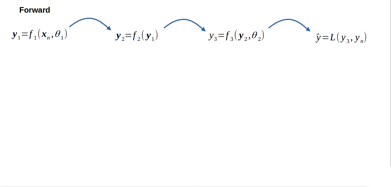

Chain rule applied to neural networks
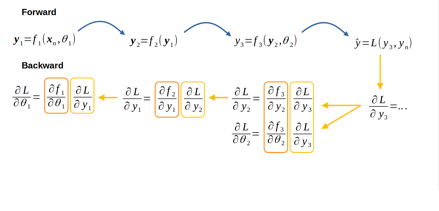

Chain rule applied to neural networks
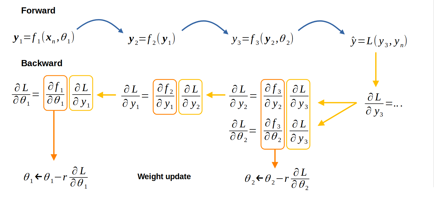

Deep learning concept

Deep learning concept


Deep learning concept


Deep learning concept
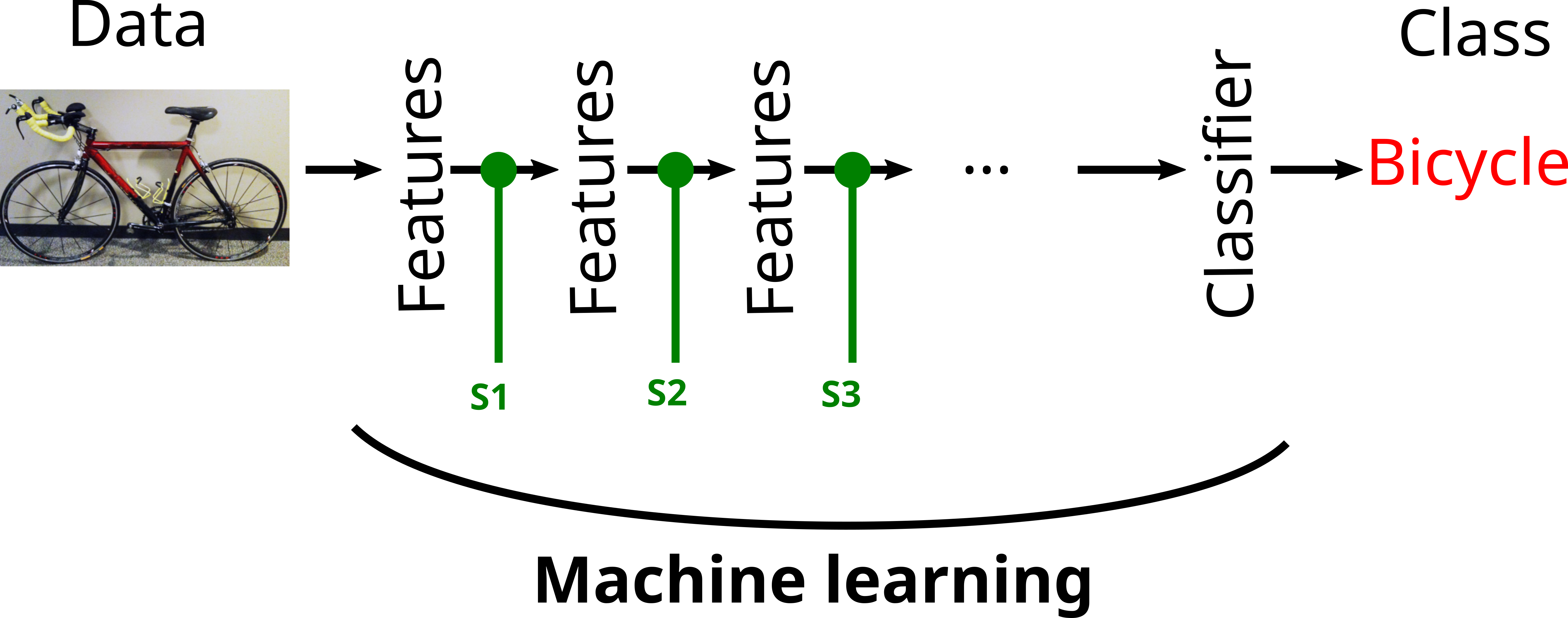

Massively data driven approaches
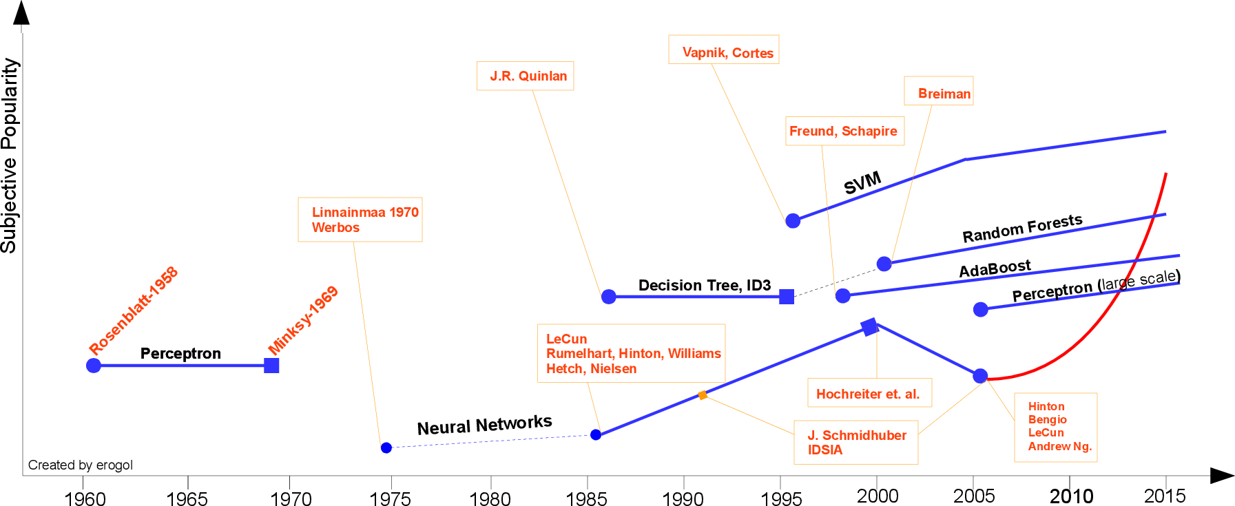

Convolutions and image processing

Multi-layer perceptron (before 1990)
MLP becomes larger and deeper
- difficult convergence
- few data
- very long training
- progessive loss of interest
SVM
- simpe to use
- convergence proof
- fast

Multi-layer perceptron for images
Using a linear layer ?
Lots of weights! (at least one per pixel!)

Multi-layer perceptron for images
Using a linear layer ?
Lots of weights! (at least one per pixel!)
Is it interesting to look at relations in the whole image ?

Convolution
Look at small neighborhoods (where the objects are)

Convolution
Look at small neighborhoods (where the objects are)
Create neurons that take a patch input

Convolution
Problem
Translation of the object must lead to same behaviour of the neurons

Convolution
Problem
Translation of the object must lead to same behaviour of the neurons
Solution
Use the same neuron (i.e. all the neurons of the layer share weights)

Convolution
Forward
Let
Then:

Convolution
Backward weight update
Let
Finally, the update rule:

Convolutions
Forward
Same with term to term multiplication:

Convolution: what do convolutions learn?
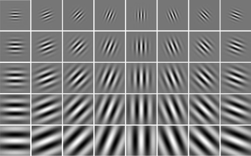
Gabor filters.
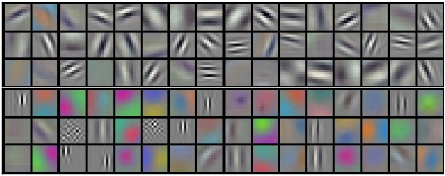
First layer of AlexNet.

Dimension reduction
With the previous convolution, the output dimension is the same as the output dimension.
For classification: only one label, need for dimension reduction.
- convolution stride: do not look at all the pixels of the input (one every two, one every three...)
- Max Pooling

Max Pooling
- dimension reduction
- relative translation invariability

Max Pooling
Forward
Max signal
Backward
Gradient transmission to max signal origin, zero otherwise

Convolutional Neural Netowkrs - LeNet (1990
Very good results on digits recognition !

Isues
Issues
- Learning speed
- Exploding or vanishing gradients
- Overfitting
- Local minima
Limitations
- Architecture
- Initialization
- Computing power
- Data
- Optimization

Solutions
- activations
- mini-batches
- batch norm
- good weight initialization
- better optimization

Activations
Rectified linear unit
- Faster gradient computation
- Similar convergence

Mini-batches
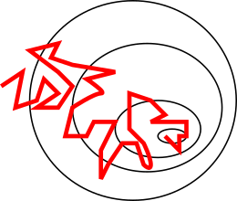
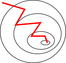
Gradient smoothing
Smoother gradient converges faster.

BatchNorm
Changes in the signal dynamic make the model more difficult to optimize: exponential or vanishing gradients.
Objective: control the signal distribution:
Learning is faster (iteration number) but slower (statistics computation).

Weight initialization
Weights have great influence on convergence speed.
They are randomly initialized.
- too small weigths: vanishing signal
- to high: exploding signal
Conservation of signal properties.

Weight initialization
Xavier initialization
finally $ Var(Y) = n Var(X_i) Var(W_i)$ and we chose

Optimization - Stochastic Gradient Descent
See neural network class
Update rule:
- Step decrease
- Exponential decrease
- Cosine annealing ...

Optimization - SGD with Momentum
Same idea as mini batch: smooth gradient in the good direction
Momentum
Use previous gradient to ponderate the direction of the new gradient.

ResNet
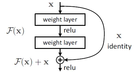


Do not forget the classics

Data
- Representative
- Data augmentation
- Data normalization

Data
Train data must be representative of the problem

Data
Data normalization
-Compute mean
-Normalize input

Data - data augmentation
Random variations of input parameters (images: lightness, contrast \dots)
- train on a more representative set
- avoid learning on unwanted features

Problems and partial solutions
Problems
- Small amount of data
- Low computational power
Solutions ?
- Use classical approaches (Perceptron, SVM, ...)